MATLAB CODE - VII

Hough-transform for Circle Detection

For detection circle with unknown radius, another parameter need to be make as variable, which is, the radius R.
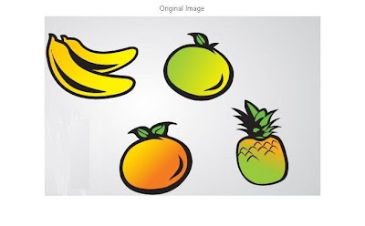
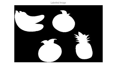
1. Reading image and the convert to binary image. After that, the location of the value '1' is found using 'find' function. (assume the image is already preprocess, if not, the 'edge' function might help)

clear all;clc;
I = imread('pic22.bmp');
I =im2bw(I);
[y,x]=find(I);
[sy,sx]=size(I);
imshow(I);


2. Find all the require information for the transformatin. the 'totalpix' is the numbers of '1' in the image.

totalpix = length(x);

3. Preallocate memory for the Hough Matrix. The R is known in the range from 1 to 50, so we reserve 50 "layers" for the HM matrix.

HM = zeros(sy,sx,50);
R = 1:50;
R2 = R.^2;
sz = sy*sx;

4. Performing Hough Transform. Notice the accumulator is located in the inner for loop.

for cnt = 1:totalpix
for cntR = 1:50
b = 1:sy;
a = (round(x(cnt) - sqrt(R2(cntR) - (y(cnt) - [1:sy]).^2)));
b = b(imag(a)==0 & a>0);
a = a(imag(a)==0 & a>0);
ind = sub2ind([sy,sx],b,a);
HM(sz*(cntR-1)+ind) = HM(sz*(cntR-1)+ind) + 1;
end
end

5. Find for the maximum value for each layer, or in other words, the layer with maximum value will indicate the correspond R for the circle.

for cnt = 1:50
H(cnt) = max(max(HM(:,:,cnt)));
end
plot(H,'*-');



6. Extract the information from the layer with maximum value, and overlap with the original image.

[maxval, maxind] = max(H);
[B,A] = find(HM(:,:,maxind)==maxval);
imshow(I); hold on;
plot(mean(A),mean(B),'xr')
text(mean(A),mean(B),num2str(maxind),'color','green')


7. This example use the "for loop" extensively, and the speed of the program is rather slow. Vectorized the code might speed up the execution time.



Measuring Object Length (with a Reference Object)

Let's see this simple example:

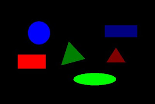
1. Reading image and show the true color image.

clear all;clc;
I = imread('pic29.tif');
imshow (I);



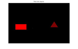
2. Assuming that we know the length of the red object (as reference) which is 5 cm, locate the red object with simple command and find the length in pixels:



Ired_labeled = bwlabel(Ired);
Ired_props = regionprops(Ired_labeled);
Ired_length_in_pixel = Ired_props.BoundingBox(3);
disp(Ired_length_in_pixel);

212

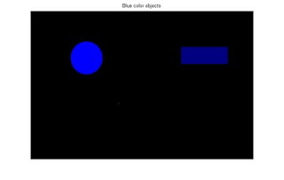
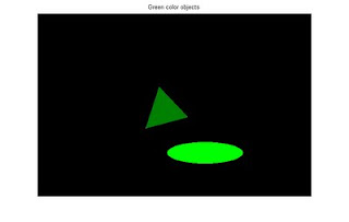
3. To measure the length of the green object, extract the object:

Igreen_labeled = bwlabel(Igreen);
Igreen_props = regionprops(Igreen_labeled);
Igreen_length_in_pixel = Igreen_props.BoundingBox(3);
disp(Igreen_length_in_pixel);

146


4. Calculate the length of green object in cm

Igreen_length_in_cm = Igreen_length_in_pixel/Ired_length_in_pixel*5;
disp(Igreen_length_in_cm);

3.4434

Neural network matlab Code

Examples of neural network using matlab

Neural Network tool is one of the toolbox in matlab. Neural Network operates Artificial intelligence approach. Most research works are used this concept.This concept mostly working in pattern recognition,classification and prediction.We give some notes, how to use neural network in matlab.

Matlab is Research tool ,mainly used for research and researchers.you have use following operations for study the Neural Network.

Neural Network contain Three layers.

1. Input Layer
2. Hidden Layer
3. Output Layer

Use following operation in Matlab for train the data on NeuralNetwork.

1. Goto matlab command window.
2. Type nftool (nftool is keyword, for load the Neural network Toolbox on matlab).
3. Then you sea following screen.

4. Load The data s from work space.

5.Set The hidden layers of neural network.

5.Then goto Next.Then press Train button train your data.

6.Then goto 2 Next Button then press generate m file.This m file is your training file.

This method for directly using Neural Network Toolbox.

In below create Neural network with using NN toolbox codes and syntax's.

1. Training use as following code

>> input_data = [1 2;2 3;2 2;4 2;6 6]; % Input matrix

>> output_data = [3;5;4;6;12]; %output vector

>> net = newff(input_data',output_data',20); % design a NN Structure

>> net = train(net,input_data',output_data');% Train the data's

2. Test the data's on NN.

>> pred = sim(net,[2;3]) % test the data's on neural network

 

pred =4.95

This "sim" is a function ,for test the data's on networks.you may have use large amount of data's to train and test on neural network

 

Tips For Research Scholars

Tips For Research Scholars | Pre-PhD Tips | Publishing Research Papers Tips 

Most of the research peoples struggle in them research.Here we put some simple tips for Research scholar.Please note this points for all per-research scholars.Very simple points for Research.

Select your Research Area

This is your most important things of your research.you have choose most like,interested and well knows domain areas.If you choose well know research area means you can easy to complete your PhD.Research area's are like networking,cloud computing or any area.

Find problem

Here you Find out the any one problem of your selected research area.You must implement and solve this problem on your research.Refer more tools and paper (most recent) for solve the find-out problem on your domain.You may use Google scholar and Microsoft research site for help your research works.you have easy to pick the research papers from these sites.

Problem Solving

In this section you must implement your research work and solve the problem  by yourself. Then you have do comparison with old algorithm and proposed algorithms.then you put the more intermediate result on your research paper.


Publishing Papers

This one is main important for you research. Most universities are want to publishing papers on best journals.so you careful to choose the Journal. if your papers accepted on Journals then Reviewer may give some tips for improve the quality of your research papers or ask some doubts of your research works,If they have any doubts then you must clarify all of doubts.If you solve all problems then your papers publishing on that Journal. otherwise may be rejected.

 

MATLAB CODING - PART VI

Fuzzy Logic Examples using Matlab,Fuzzy Logic Modeling with Matlab,Introduction to Fuzzy Logic using MATLAB

Fuzzy Logic, which used in Artificial intelligence.It contain logical think of rules and member input and output functions. Three steps are taken to generate a fuzzy control engine:

1)Fuzzification(Using membership functions to graphically illustrate a situation)
2)Rule evaluation(purpose of fuzzy rules)
3)Defuzzification(find the crunchy or actual results)

Here we provide the examples of Fuzzy Logic and design it.In below one way you easy create the Fuzzy project using matlab tool.

In Matlab contain a fuzzy Toolbox.it simple to create an Fuzzy Logic.
1.Type fuzzy in matlab command prompt.

2.Add a input and output variables.

in coding as follows

a = newfis('my_fis');
a = addvar(a,'input','service',[0 10]);
a = addmf(a,'input',1,'poor','gaussmf',[1.5 0]);
a = addmf(a,'input',1,'good','gaussmf',[1.5 5]);
a = addmf(a,'input',1,'excellent','gaussmf',[1.5 10]);

3.Set the input variable range and corresponding input membership function ranges,same thing do in output also.

4.choose type of Mf functions.

5.Double click the mamdani for adding a rules.

in coding

ruleList=[1 1 1 1 1
1 2 2 1 1];

a = addrule(a,ruleList);

In ruleList 1st row is 1st rule.in first 3 ones are input range and output range.in 4 is and /or 5 th one is weight of the rule.

6.Finaly save that fuzzy file name on your hard disk.

Testing a Fuzzy

1. Load a my_fis.fis in matlab command window using following commands.

my_fis_mat = readfis('my_fis'); % reading fis file

2.Give the inputs.

If you have two input means give two values in one vector array.
test_data is

my_fis_mat = readfis('my_fis');
my_test = [2 1; 4 9];
out = evalfis(my_test,my_fis_mat)

in out variable contain your result of your fuzzy. Finally you got the answer.

 

MATLAB CODING - PART V

Matlab Database Connectivity Example code 

 1.Create Connection String

Connection String used to connect the database.That syntax as follows
conn_str = database('database_name','username','password','driver','database_url');
Example :
>>conn_str = database('my_db','scott','tiger','oracle.jdbc.driver.OracleDriver','jdbc:oracle:oci7:');

Here we create the connection string on Oracle database.Like you connect different type of  databases.

2.Execute Query String on Database

exec function to execute the query strings on database.Syntax as follows

curs = exec(conn_str, 'sql_query');

Example :

>>curs = exec(conn_str, 'Select * from My_Table');

 

 above example retrieve the all data's from My_Table.Like you do execute all type of sql queries.

3.Fetch the cursor to a MATLAB variable 

Here we convert the cursor data into matlab variable. example code as below

>>my_data = fetch(curs);

Finally my_data contain all data's of My_Table.

 

Matlab read raw file example code , Matlab convert raw file to Jpg example

 To convert raw file to Jpg image file example code.In raw file contain slices images . raw format is one of the image compress format.
code :

f=fopen('t1_icbm_normal_1mm_pn3_rf20.rawb');
a=fread(f);
input_img = reshape(a,181,217,181);
[r c m] = size(input_img);

for i = 1 : m
imwrite(input_img(:,:,i),['img_' num2str(i)],'jpg')
figure,imshow(uint8(input_img(:,:,i)));
end

In above code convert raw file to Jpg image file then write the image on current directory and show the each slice images.

MATLAB CODING - PART IV

The information hiding homepage Digital watermarking & steganography

Matlab code

Hare = imread('arctic_hare.bmp', 'bmp');
F15 = imread('F15.bmp', 'bmp');
n = 4; % Number of bits to replace 1 <= n <= 7

[Stego, Extracted] = LSBHide(Hare, F15, n);

figure, imshow(Stego)
figure, imshow(Extracted)

where

function [Stego, Extracted] = LSBHide(Cover, Hidden, n)
%LSBHide
% [Stego, Extracted] = LSBHide(Cover, Hidden, n)
% Hide Hidden in the n least significant bits of Cover

Stego = uint8(bitor(bitand(Cover, bitcmp(2^n - 1, 8)) , bitshift(Hidden, n - 8)));
Extracted = uint8(bitand(255, bitshift(Stego, 8 - n)));

MATLAB CODING'S - PART III

Correcting Nonuniform Illumination

This example shows how to correct nonuniform illumination in an image to make it easy to identify individual grains of rice in the image. You can then learn about the characteristics of the grains and easily compute statistics for all the grains in the image.

Step 1: Read Image

I = imread('rice.png');
imshow(I)

Step 2: Use Morphological Opening to Estimate the Background

Notice that the background illumination is brighter in the center of the image than at the bottom. Use imopen to estimate the background illumination.

background = imopen(I,strel('disk',15));

% Display the Background Approximation as a Surface
figure, surf(double(background(1:8:end,1:8:end))),zlim([0 255]);
set(gca,'ydir','reverse');

Step 3: Subtract the Background Image from the Original Image

I2 = I - background;
imshow(I2)

Note that step 2 and step 3 together could be replaced by a single step using imtophat which first calculates the morphological opening and then subtracts it from the original image.
I2 = imtophat(I,strel('disk',15));

Step 4: Increase the Image Contrast

I3 = imadjust(I2);
imshow(I3);

Step 5: Threshold the Image

Create a new binary image by thresholding the adjusted image. Remove background noise with bwareaopen.

level = graythresh(I3);
bw = im2bw(I3,level);
bw = bwareaopen(bw, 50);
imshow(bw)

Step 6: Identify Objects in the Image

The function bwconncomp finds all the connected components (objects) in the binary image. The accuracy of your results depend on the size of the objects, the connectivity parameter (4,8,or arbitrary), and whether or not any objects are touching (in which case they may be labeled as one object). Some of the rice grains in bw are touching.

cc = bwconncomp(bw, 4)

cc = 

    Connectivity: 4
       ImageSize: [256 256]
      NumObjects: 95
    PixelIdxList: {1x95 cell}

Step 7: Examine One Object

Each distinct object is labeled with the same integer value. Show the grain that is the 50th connected component.

grain = false(size(bw));
grain(cc.PixelIdxList{50}) = true;
imshow(grain);

Step 8: View All Objects

One way to visualize connected components is to create a label matrix and then display it as a pseudo-color indexed image.
Use labelmatrix to create a label matrix from the output of bwconncomp. Note that labelmatrix stores the label matrix in the smallest numeric class necessary for the number of objects.

labeled = labelmatrix(cc);
whos labeled

  Name           Size             Bytes  Class    Attributes

  labeled      256x256            65536  uint8              

In the pseudo-color image, the label identifying each object in the label matrix maps to a different color in the associated colormap matrix. Use label2rgb to choose the colormap, the background color, and how objects in the label matrix map to colors in the colormap.

RGB_label = label2rgb(labeled, @spring, 'c', 'shuffle');
imshow(RGB_label)

Step 9: Compute Area of Each Object

Each rice grain is one connected component in the cc structure. Use regionprops on cc to get the area.

graindata = regionprops(cc,'basic')

graindata = 

95x1 struct array with fields:
    Area
    Centroid
    BoundingBox

To find the area of the 50th component, use dot notation to access the Area field in the 50th element of graindata structure array.

graindata(50).Area

ans =

   194

Step 10: Compute Area-based Statistics

Create a new vector allgrains, which holds the area measurement for each grain.

grain_areas = [graindata.Area];

Find the grain with the smallest area.

[min_area, idx] = min(grain_areas)
grain = false(size(bw));
grain(cc.PixelIdxList{idx}) = true;
imshow(grain);

min_area =

    61


idx =

    16

Step 11: Create Histogram of the Area

nbins = 20;
figure, hist(grain_areas,nbins)
title('Histogram of Rice Grain Area');

 

MATLAB CODING'S - PART II

Auto Cropping- Based on labeling the connected components 

 This post is about labeling the connected components in a binary image and crop the connected components based on the label. The main two functions used for this simple operation are ‘bwlabel’ and ‘regionprops’. 

  I used ‘bwlabel’ to label the connected components.  After labeling, I used ‘regionprops’ function to find the rectangle containing the region.  To find the rectangle points, I used ‘BoundingBox’ property.Then the labeled components are automatically cropped and the image is displayed. To crop an image, ‘imcrop’ function is used.

MATLAB CODE:

A=imread('coins.png');
figure,imshow(A); title('Original Image');

                                 

%Convert the Image to binary
B=im2bw(A);
 
%Fill the holes
C=imfill(B,'holes');
 
%Label the connected components
[Label,Total]=bwlabel(C,8);
figure,imshow(C); title('Labelled Image');

Add caption

%Rectangle containing the region
Sdata=regionprops(Label,'BoundingBox');
 
%Crop all the Coins 
for i=1:Total
    Img=imcrop(A,Sdata(i).BoundingBox);
    Name=strcat('Object Number:',num2str(i));
    figure,imshow(Img); title(Name);
end

Add caption

Another Example:

'coins.png'

Labeled Image

Bit-Plane Slicing 

Digitally, an image is represented in terms of pixels.

These pixels can be expressed further in terms of bits.

Consider the image ‘coins.png’ and the pixel representation of the image.

Consider the pixels that are bounded within the yellow line. The binary formats for those values are (8-bit representation)

The binary format for the pixel value 167 is 10100111

Similarly, for 144 it is 10010000

This 8-bit image is composed of eight 1-bit planes.

Plane 1 contains the lowest order bit of all the pixels in the image.

And plane 8 contains the highest order bit of all the pixels in the image.

Let’s see how we can do this using MATLAB

A=[167 133 111

      144 140 135

      159 154 148]

B=bitget(A,1);  %Lowest order bit of all pixels

‘bitget’ is a MATLAB function used to fetch  a bit from the specified position from all the pixels.

B=[1 1 1

      0 0 1

      1 0 0]

B=bitget(A,8);%Highest order bit of all pixels

B=[1 1 0

      1 1 1 

      1 1 1]

MATLAB CODE:

%Bit Planes from 1 to 8. Output Format: Binary

A=imread('coins.png');

B=bitget(A,1);

figure,

subplot(2,2,1);imshow(logical(B));title('Bit plane 1');

B=bitget(A,2);

subplot(2,2,2);imshow(logical(B));title('Bit plane 2');

B=bitget(A,3);

subplot(2,2,3);imshow(logical(B));title('Bit plane 3');

B=bitget(A,4);

subplot(2,2,4);imshow(logical(B));title('Bit plane 4');

 

B=bitget(A,5);

figure,

subplot(2,2,1);imshow(logical(B));title('Bit plane 5');

B=bitget(A,6);

subplot(2,2,2);imshow(logical(B));title('Bit plane 6');

B=bitget(A,7);

subplot(2,2,3);imshow(logical(B));title('Bit plane 7');

B=bitget(A,8);

subplot(2,2,4);imshow(logical(B));title('Bit plane 8');

 

Image reconstruction using n bit planes.

1.     The nth plane in the pixels are multiplied by the constant 2^n-1

2.     For instance, consider the matrix

A= A=[167 133 111

      144 140 135

      159 154 148] and the respective bit format

         

3.     Combine the 8 bit plane and 7 bit plane.

For 10100111, multiply the 8 bit plane with 128 and 7 bit plane with 64.

(1x128)+(0x64)+(1x0)+(0x0)+(0x0)+(1x0)+(1x0)+(1x0)=128

4.     Repeat this process for all the values in the matrix and the final result will be

[128 128 64

 128 128 128

128 128 128]

MATLAB CODE:

%Image reconstruction by combining 8 bit plane and 7 bit plane

A=imread('coins.png');

B=zeros(size(A));

B=bitset(B,7,bitget(A,7));

B=bitset(B,8,bitget(A,8));

B=uint8(B);

figure,imshow(B);

Image reconstructed using 8 and 7 bit planes

Explanation:

‘bitset’ is used to set  a bit at a specified position. Use ‘bitget’ to get the bit at the positions 7 and 8 from all the pixels in matrix A and use ‘bitset’ to set these bit values at the positions 7 and 8 in the matrix B.

%Image reconstruction by combining 8,7,6 and 5 bit planes

A=imread('coins.png');

B=zeros(size(A));

B=bitset(B,8,bitget(A,8));

B=bitset(B,7,bitget(A,7));

B=bitset(B,6,bitget(A,6));

B=bitset(B,5,bitget(A,5));

B=uint8(B);

figure,imshow(B);

Image reconstructed using 5,6,7 and 8 bit planes

Find Area, Perimeter, Centroid, Equivdiameter, Roundness and Bounding Box without Using MATLAB Function ‘regionprops’ 

 

In MATLAB, the function ‘regionprops’ is used to measure the image properties. Here are some basic properties computed without using the function.

          Read an image and find the connected components using ‘bwlabel’ function.

Using the Labeled matrix as an input, the properties can be measured.

Example:

A=[1 0 0 1

      1 1 1 1

      0 0 1 1]

To find Area:

·        The total number of ‘ON’ pixels in the image.

The number of ones in the matrix is 8.

              

To find Centroid:

·        Find the row and column having pixel value one. Eg.[row,column]=find(label==1)

Row=[ 1     2     2     2     3     1     2     3]

Column=[ 1     1     2     3     3     4     4     4]

·        Find the mean of the row and column having pixel value one.

Mean of Row=2 and mean of column= 2.75

To find the Bounding Box:

·        We need 4 points, starting position(x,y) , length and breadth.

·        Minimum value of row and column minus 0.5 gives starting position(x,y) respectively

·        Minimum value of  row=1-0.5=0.5

·        Minimum value of column=1-0.5=0.5

·        Maximum value of column – minimum value of column+1 gives breadth of the box

·        Maximum value of column=4

·        Max value-min value of column=3+1

·        Maximum value of row- minimum value of row +1gives length of the box

·        maximum value of row=3

·        Max value – Min value=2+1

·        Bounding Box value for the given example:0.5000    0.5000    4.0000    3.0000

·        For more details on how to draw a rectangle check here: http://angeljohnsy.blogspot.in/2011/06/how-to-draw-in-matlab.html

To find the Perimeter

·        Find the boundary of the labeled component

Boundary pixels:

     1     1

     2     2

     2     3

     1     4

     2     4

     3     4

     3     3

     2     2

     2     1

     1     1

·        Find the distance between the each adjoining pair of pixels around the border of the region.

·        Use the distance formula:

                                             

·        For instance, calculate the distance between the two points (1,1) and (2,2). distance=sqrt((2-1).^2+(2-1).^2)=1.41

·        Similarly, the distance is computed for all the pixel positions.

·        The perimeter for the given example is 10.2426

To find the Roundness:

·        Roundness of  an object can be determined using the formula: 

     Roundness=(4*Area*pi)/(Perimeter.^2) 
        If the Roundness is greater than 0.90 then, the object is circular in shape.

     Result= (4*8*3.14)/10.2426.^2=0.9582
           

To find the Equivdiameter

·        Formula: sqrt(4*Area/pi).

     Equivdiameter for the given example:3.1915

   

 

MATLAB - CODING'S

Identifying Objects based on color (RGB) 

A bitmap image with different shapes filled with primary colors Red, Blue and Green.The objects in the image are separated based on the colors. The image is a RGB image which is a 3 dimensional matrix.

Lets use (i,j) for getting the pixel position of the image A.

In the image, A (i, j, 1) represents the value of red color.

 A (i, j, 2) represents the green color.

A (i, j, 3) represents the blue color.

To separate the objects of color red:

Check if A (i, j, 1) is positive. [In most cases the value will be 255];

 A (i, j, 2) and A (i, j, 3) will be zero.

Similarly, other colors can be separated.

MATLAB CODE:

A=imread('shapes.bmp');

figure,imshow(A);

title('Original image');

%Preallocate the matrix with the size of A

Red=zeros(size(A));

Blue=zeros(size(A));

Green=zeros(size(A));

for i=1:size(A,1)

    for j=1:size(A,2)

       

        %The Objects with Red color

        if(A(i,j,1) < = 0)

          Red(i,j,1)=A(i,j,1);

          Red(i,j,2)=A(i,j,2);

          Red(i,j,3)=A(i,j,3);

        end

       

        %The Objects with Green color

        if(A(i,j,2) < = 0)

          Green(i,j,1)=A(i,j,1);

          Green(i,j,2)=A(i,j,2);

          Green(i,j,3)=A(i,j,3);

        end

       

        %The Objects with Blue color

        if(A(i,j,3) < = 0)

          Blue(i,j,1)=A(i,j,1);

          Blue(i,j,2)=A(i,j,2);

          Blue(i,j,3)=A(i,j,3);

        end

       

    end

end

Red=uint8(Red);

figure,imshow(Red);

title('Red color objects');

            

Blue=uint8(Blue);

figure,imshow(Blue);

title('Blue color objects');

             

                 

Green=uint8(Green);

figure,imshow(Green);

title('Green color objects');

Identifying the objects based on count(bwlabel) 

Steps To Be Performed:

1. Convert the RGB image to binary image.
2. Fill the holes in the image.
3. Label the objects in the image based on connectivity 8
4. Display the images in a RGB format

4.1.  Store the co-ordinates(x,y) of the object 1 which is  labeled as 1.

4.2.  Calculate the image size for object one. The length can be found by subtracting the maximum and the minimum of y values. Similary for x find the width by subtracting the maximum and minimum of x values.

4.3.  Now map the pixel value to the new image.

A=imread('num2.jpg');

figure,imshow(A);

title('Original image');

C=~im2bw(A);

B=imfill(C,'holes');

label=bwlabel(B,8);

for j=1:max(max(label))

[row, col] = find(label==j);

len=max(row)-min(row)+2;

breadth=max(col)-min(col)+2;

target=uint8(zeros([len breadth 3] ));

sy=min(col)-1;

sx=min(row)-1;

for i=1:size(row,1)

    x=row(i,1)-sx;

    y=col(i,1)-sy;

    target(x,y,:)=A(row(i,1),col(i,1),:);

end

mytitle=strcat('Object Number:',num2str(j));

figure,imshow(target);title(mytitle);

end

The objects that are displayed in a RGB format.